Intuitively Understanding Harris Corner Detector
If you ever tried to learn how the Harris corner detection algorithm works, you might have noticed that the process is not intuitive at all. First, you start with an energy function, approximate it using Taylor approximation, get a matrix from that, then find the eigenvalues of that matrix, etc. But when you come to the final implementation, it is rather simple and seems easier. If you are like me, this is not intuitive at all. But today I will present you a much easier way to understand how the Harris corner detection algorithm works.
Let’s start with understanding what is a corner. We can simply think of it as a connection of edges. For two edges to be able to connect, they sure need to be not parallel, so looking at a corner, we should see that edges moving in different directions (they would be parallel if they moved in the same directions):
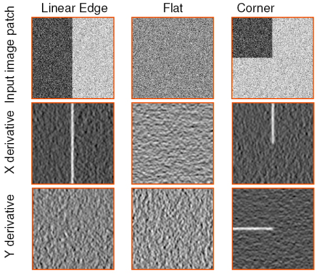
Figure source: https://www.cse.psu.edu/~rtc12/CSE486/lecture06.pdf
So it is obvious that the gradients of the image Ix and Iy will both be active in the corner region. We know that adding Ix2 and Iy2 shows the regions with change in x or y directions (which is the basis of the all edge detection algorithms). So one thing that comes to mind is multiplying the Ix2 and Iy2 so that we will only see regions on the image that have a change in both x and y directions at the same time, just like corners!
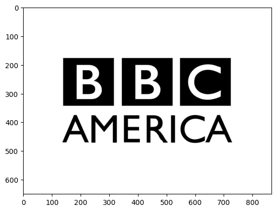
Let’s start implementing this. First, let’s find a pretty basic image that will have lots of corners inside it.
import cv2
import matplotlib.pyplot as plt

# wget https://logowik.com/content/uploads/images/bbc-america9038.jpg -O assets/bbc.jpg

img = cv2.imread("assets/bbc.jpg", cv2.IMREAD_GRAYSCALE)
plt.imshow(img, cmap="gray")
Now we can start finding the gradient of this image using the Sobel operator:
Ix = cv2.Sobel(img, ddepth=cv2.CV_32F, dx=1, dy=0)
Iy = cv2.Sobel(img, ddepth=cv2.CV_32F, dx=0, dy=1)
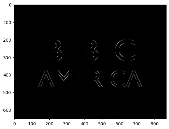
Okay, we are there now. Let’s plot the Ix2Iy2, we are expecting it to give us regions with both x and y directions:
plt.imshow(Ix**2 * Iy**2, cmap='gray')

As you can see, we are kind of not successful, because this shows us the both corners and edges that move along in both x and y directions. But we need to get rid of the edges.
If you carefully look at this resulting image, you will notice that corners are either isolated like the top left corner of the B logo, or they are at the end of these edges. Maybe we can’t get rid of the edges directly, but if somehow we can remove the corners from Ix2Iy2, we can subtract it from the original Ix2Iy2 and get only the corners. Actually, we can get rid of the corners. Since the corners are isolated in this image, applying a Gaussian blur will decrease the intensities of the corners a lot!
Let’s see this:
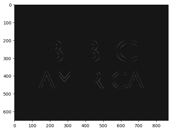
corners_suppressed = cv2.GaussianBlur(Ix**2 * Iy**2, ksize=(0, 0), sigmaX=1)
plt.imshow(corners_suppressed, cmap='gray')

We can even do a better job of removing the corners by applying the blur before squaring. Because square will increase the intensity of isolated corners, making it less affected by the blur. So we can instead do:
corners_suppressed = cv2.GaussianBlur(Ix* Iy, ksize=(0, 0), sigmaX=1) ** 2
plt.imshow(corners_suppressed, cmap='gray')
Now that we have the corners mostly suppressed image, we can try subtracting this from the Ix2Iy2 and get only the corners. Let’s try it:
plt.imshow(Ix**2 * Iy**2 - corners_suppressed, cmap='gray')
That doesn’t seem to work, but the reason is clear. Edges of the Ix2Iy2
have different intensity than corners_suppressed, since corners_suppressed has been blurred.
We want them to have the same intensity in edges so that they cancel the edges when they are subtracted.
We can make the edges of Ix2Iy2 similar intensity to edges of corners_suppressed
by applying Gaussian blur to Ix2 and Iy2 seperately before multiplying them.
We will apply the blur to squared gradients to make sure the corners are less affected by the blur.
Ix_squared = cv2.GaussianBlur(Ix**2, ksize=(0, 0), sigmaX=1)
Iy_squared = cv2.GaussianBlur(Iy**2, ksize=(0, 0), sigmaX=1)

corners = Ix_squared * Iy_squared - corners_suppressed
plt.imshow(corners, cmap='gray')
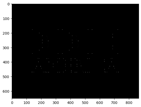
Yes! We successfully get the corners of the image. Now if we look at the data inside the corners matrix, you will notice that
corners have extremely large values and other parts have smaller values. Let’s threshold it:
corners[corners < corners.max() / 5] = 0
corners[corners != 0] = 255

plt.imshow(corners, cmap="gray")

Okay, let’s plot these points as circles in our image:
new_img = cv2.cvtColor(img, cv2.COLOR_GRAY2RGB)

for i in range(img.shape[0]):
    for j in range(img.shape[1]):
        if corners[i][j] == 255:
            cv2.circle(new_img, (j, i), radius=2, color=(255, 0, 0), thickness=-1)

plt.imshow(new_img, cmap="gray")
plt.show()
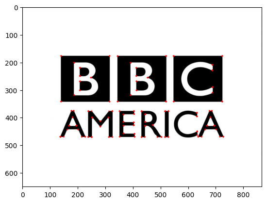
And with this, we have implemented the Harris corner detection algorithm and we haven’t talked about things like fitting ellipses, Taylor series approximation, or any of that stuff. This implementation is equivalent to the other implementations of this algorithm.
Here is the full code:
import cv2
import matplotlib.pyplot as plt

# wget https://logowik.com/content/uploads/images/bbc-america9038.jpg -O assets/bbc.jpg

img = cv2.imread("assets/bbc.jpg", cv2.IMREAD_GRAYSCALE)

Ix = cv2.Sobel(img, ddepth=cv2.CV_32F, dx=1, dy=0)
Iy = cv2.Sobel(img, ddepth=cv2.CV_32F, dx=0, dy=1)

corners_suppressed = cv2.GaussianBlur(Ix* Iy, ksize=(0, 0), sigmaX=1) ** 2
Ix_squared = cv2.GaussianBlur(Ix**2, ksize=(0, 0), sigmaX=1)
Iy_squared = cv2.GaussianBlur(Iy**2, ksize=(0, 0), sigmaX=1)

corners = Ix_squared * Iy_squared - corners_suppressed
corners[corners < corners.max() / 5] = 0
corners[corners != 0] = 255

new_img = cv2.cvtColor(img, cv2.COLOR_GRAY2RGB)

for i in range(img.shape[0]):
    for j in range(img.shape[1]):
        if corners[i][j] == 255:
            cv2.circle(new_img, (j, i), radius=2, color=(255, 0, 0), thickness=-1)

plt.imshow(new_img, cmap="gray")
plt.show()
Hopefully, you now understand how this algorithm works and enjoy the process.