Understanding and Building Neural Networks: A Step-by-Step Guide from Scratch
In this tutorial, we will learn two different methods to implement neural networks from scratch using Python:
- Extremely simple method: Finite difference
- Still a very simple method: Backpropagation
There are many tutorials about neural networks, but I bet this is the most intuitive one. We will not be calculating derivatives by hand like most of them are doing, and we will understand the core concept behind gradient descent algorithm by seeing how things work with the finite difference method, not just memorize it.
The implementation will start very basic and we will build on top of it slowly so that you will understand every part of the process.
In the end, we will have the code to train neural networks to predict AND and XOR. If you don’t know what they are, don’t worry, they are super basic. You will understand it when we come to that part. But know that our implementation at the end will be able to learn much more complex structures than such binary gates.
But let’s start with understanding the high-level concept behind neural networks. They have the following steps:
- Create your network with trainable parameters
- Run your neural network and get your output, let’s call it the prediction
- Based on this prediction and the value it should actually be, calculate the loss (test how bad the network is at predicting)
- Find the derivatives of the loss function for its parameters
- Update the parameters by subtracting their scaled derivatives
And repeat these steps until you are happy with the predictions of your neural network.
These steps will look something like this in the code:
model = NN()                           # 1

while you_are_not_happy:
    prediction = model(x)              # 2
    loss = (prediction - y) ** 2       # 3
    loss.backward()                    # 4

    for p in model.parameters:
        p.value -= lr * p.grad         # 5
Look’s pretty easy, huh? Let’s go step by step:
1. Create your neural network with trainable parameters
The definition of neural networks can be very broad, but for learning purposes let’s imagine it as a function that takes
a number input of any size, and multiplies it with some parameters. These parameters are just randomly initialized
numbers.
The key part here is that after this step,
you process the results with some kind of a non-linear function, and re-iterate these steps many times
with different parameters.
It can be a little bit hard to understand this concept, but it is actually very simple. You’ll see how simple it is when you see the code for it. However, you should note that the number of parameters depends on the data you will feed. Consider we are trying to learn the AND gate. If you don’t know what it is, you can think of it as a function that takes two values, 0 or 1 and returns 0 if any of the inputs is 0, and 1 otherwise. It looks like this:
| p | q | p&q |
|---|---|---|
| 0 | 0 | 0 |
| 0 | 1 | 0 |
| 1 | 0 | 0 |
| 1 | 1 | 1 |
Now let’s get back to the neural networks. We want the network to learn p&q given p and q values. Here is an architecture for this task:
import random

class NN:
    def __init__(self):
        self.parameter1 = random.random()
        self.parameter2 = random.random()

    def forward(self, p, q):
        out1 = p * self.parameter1
        out2 = q * self.parameter2
        output = out1 + out2

        return output
This is extremely simple! But it’s not very capable of learning. This is because we missed some key functionalities. One of them is that we need a non-linear function, also known as activation function.
There are several very popular candidates for it and you may have heard of them before, like Sigmoid, TanH and ReLU functions. Let’s learn about the sigmoid.
A sigmoid function is a function that given any value, squashes it to be between 0 and 1. If you feed a very big number like 46598, it will give almost 1 and if you feed -73412, it will give almost 0. For input 0 it will give 0.5. This function looks something like this:
\[\sigma(x) = \frac{1}{1+e^{-x}}\]If we plot it, it will look like:
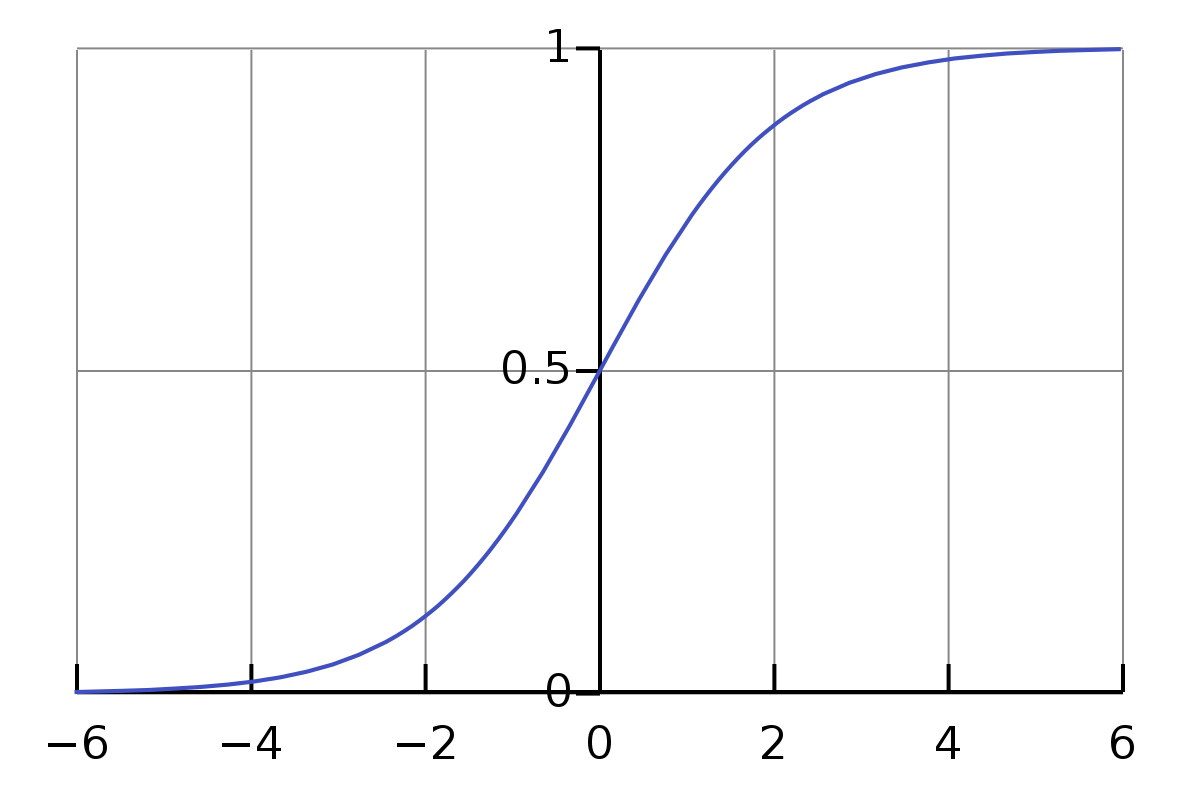
This function may seem complicated, but the intuition behind is very simple, just squash the numbers to be between 0 and 1. This is a very popular activation function used in lots of places. There are more modern alternatives exist, but we will stick with this for now.
Now let’s implement and use it:
import random
import math

class NN:
    def __init__(self):
        self.parameter1 = random.random()
        self.parameter2 = random.random()

    def sigmoid(self, x):
        return 1 / (1 + math.exp(-x))

    def forward(self, p, q):
        out1 = p * self.parameter1
        out2 = q * self.parameter2
        output = self.sigmoid(out1 + out2)

        return output
This is great and we are almost done with the definition of our Neural Network. But one more thing we will be adding to it: Another parameter that we will use to add instead of multiplying. The only reason we add one more parameter is to increase the capabilities of our network. The more operations it can do, the more things it can learn!
We will add this parameter to the multiplication result:
import random
import math

class NN:
    def __init__(self):
        self.parameter1 = random.random()
        self.parameter2 = random.random()
        self.parameter3 = random.random()

    def sigmoid(self, x):
        return 1 / (1 + math.exp(-x))

    def forward(self, p, q):
        out1 = p * self.parameter1
        out2 = q * self.parameter2
        output = self.sigmoid(out1 + out2 + self.parameter3)

        return output
Now our architecture is completely ready! If you ever heard of the terms weights and biases in the context of neural networks, our first two parameters are weights and the third parameter is the bias. Weights get multiplied, and biases get added.
2. Run your neural network and get your output
We have our network defined now, we can call its forward function to start getting some output. First, let’s define our data and start predicting values:
data = [
    [0, 0, 0],
    [0, 1, 0],
    [1, 0, 0],
    [1, 1, 1],
]

model = NN()

for d in data:
    bit1, bit2 = d[0], d[1]
    prediction = model.forward(bit1, bit2)

    real_value = d[2]
    print(f"predicted: {prediction}, real value: {real_value}")
If you run this you will get something like this:
predicted: 0.63, real value: 0
predicted: 0.66, real value: 0
predicted: 0.80, real value: 0
predicted: 0.82, real value: 1
Now you are seeing how bad our neural network is. It’s simply because we haven’t trained it yet.
Notice that no matter what initial parameters you set, the prediction will always be between 0 and 1 due to the sigmoid function. It squashes any number it takes.
3. Based on the prediction and the value it should actually be, calculate the loss
By loss, we mean assessing how badly our network is performing. Right now it performs very badly, so we should get a high number. To get a numeric value for that, we can sum up the differences between each prediction and it’s supposed to be real value:
loss = 0
for d in data:
    bit1, bit2 = d[0], d[1]
    prediction = model.forward(bit1, bit2)

    real_value = d[2]
    loss += (prediction - loss) ** 2
    print(f"predicted: {prediction}, real value: {real_value}")

print(f"loss: {loss}")
For the distance between prediction and real value, we used the square function. Since distance is a positive term, squaring will make the result positive.
This will give us a value like 0.64, of course depending on the initial values of parameters. If our network would managed to give perfect predictions, our loss would be 0.
4. Find the derivatives of the loss function for its parameters
Now we found the loss value and it is clear that we want it to be close to 0 as possible. The lower the loss, the better the predictions are. One way to decrease it is using the gradient descent algorithm.
Finite difference
The gradient descent algorithm requires finding the derivatives of the parameters for the loss, but this is not intuitive. Instead, we’ll learn a very intuitive way of decreasing the loss value and it would be equivalent to gradient descent algorithms used by popular frameworks like PyTorch, called finite difference.
For each parameter, we will add some small value to it and check the loss again. If the new loss is smaller, then we will change this parameter’s value in that direction. If the new loss is bigger, we will change it in the opposite direction.
You can understand this by a simple example. Let’s say you have a device to change the room’s temperature, and it is controlled by three different control knobs.

But you don’t know what they do. So you start by changing the first knob until you feel better about the temperature. Then you go on to the second knob and do this again, and for the third knob. You go through this step a couple of times, you will find the perfect conditions for you. This is actually how the gradient descent algorithm works!
Isn’t it very easy? After doing this for our parameters for many steps, we expect the loss to be a very small value.
Now we’ll implement this in Python. But first, let’s make the code so far a bit more structural to implement this easier:
import random
import math

class NN:
    def __init__(self):
        self.parameters = [random.random() for _ in range(3)]

    def sigmoid(self, x):
        return 1 / (1 + math.exp(-x))

    def forward(self, p, q):
        out1 = p * self.parameters[0]
        out2 = q * self.parameters[1]
        output = self.sigmoid(out1 + out2 + self.parameters[2])

        return output

    def calculate_loss(self, data):
        loss = 0
        for d in data:
            bit1, bit2 = d[0], d[1]
            prediction = self.forward(bit1, bit2)

            real_value = d[2]
            loss += (prediction - real_value) ** 2

        return loss


data = [
    [0, 0, 0],
    [0, 1, 0],
    [1, 0, 0],
    [1, 1, 1],
]

model = NN()
We converted the parameters into an array and we have a built-in function to calculate the loss. Now we are ready:
for _ in range(1000):
    current_loss = model.calculate_loss(data)
    print(f"loss: {current_loss}")

    changes = []
    for i in range(len(model.parameters)):
        model.parameters[i] += 1  # change the parameter a little bit
        new_loss = model.calculate_loss(data)

        change = new_loss - current_loss
        changes.append(change)

        model.parameters[i] -= 1  # restore the parameter

    for i in range(len(model.parameters)):
        model.parameters[i] -= changes[i]
        # we subtract changes[i] because if the change is positive it means we did bad
        # we want to go in the opposite direction
And here you go! You implemented your first neural network. Now if you run this you’ll see that the loss will be almost 0 by the end of the loop. We can then test the predictions of the network:
for d in data:
    bit1, bit2 = d[0], d[1]
    prediction = model.forward(bit1, bit2)

    print(f"{bit1} & {bit2} = {prediction}")
You’ll see you get almost correct results. For 1 & 1, it will give something like 0.95 but you can always round it :)
Now what we actually did was approximating the derivatives. Derivative means change and this is what we have done. In fact, the mathematical definition of derivative is:
\[L = \lim_{h \rightarrow 0} \frac{f(a+h) - f(a)}{h}\]And if you set h to 1, you get:
\[L \approx f(a+1) - f(a)\]Which is exactly what we did! We increased the parameter by one and looked at the difference. Then we used it as our derivative.
But your instincts might have said 1 is too big of a value to add when you saw the code. And you are right. We should use a lower value and as the definition of derivative says, we should divide by that number also:
for _ in range(1000):
    current_loss = model.calculate_loss(data)
    print(f"loss: {current_loss}")

    derivatives = []
    eps = 0.0001 # think of eps as the h
    for i in range(len(model.parameters)):
        model.parameters[i] += eps  # change the parameter a little bit
        new_loss = model.calculate_loss(data)

        derivative = (new_loss - current_loss) / eps
        derivatives.append(derivative)

        model.parameters[i] -= eps  # restore the parameter

    for i in range(len(model.parameters)):
        model.parameters[i] -= derivatives[i]
        # we subtract changes[i] because if the change is positive it means we did bad
        # we want to go in the opposite direction
Now we are talking! This is a valid gradient descent algorithm implemented and you can see that it works.
But this algorithm has two very big disadvantages:
- It will be very slow as it requires computing loss again and again for each parameter change. We can have millions of parameters
- For complex networks, we may need to decrease the h value further for best derivative approximation, but we can only go up to a point since computers can work up to a certain precision
Backpropagation
Instead of the finite difference, we will use a different algorithm called backpropagation to calculate the derivatives which is also very simple. To understand it, we should first understand the concept of computation graphs.
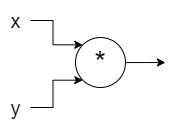
A computation graph is simply a graph of operations where each node is an operation and edges represent values.
Graph for x * y looks like:
Or a more complicated operation:
\[(x^2 + 3) ^ 2 + y\]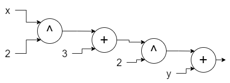
As it can be seen, it’s just writing the operations differently. But the magical thing about computation graphs is that it can help us to find the derivatives easily for any function. Let’s see the process first and understand how it works later on.
First, for each edge coming to an operation node, we write the derivative of that operation on top of it. The cool part is that we don’t need to find the gradients up until that point. For example, if we want to find the derivative of a+b, there will be a single operation node and each edge will get 1 as:
\[\frac{\partial (a+b)}{\partial a} = 1\ \ \ \ \ \ \ \ \ \frac{\partial (a+b)}{\partial b} = 1\]We can also write it for multiplication and power operations, which is necessary for us to know. But we don’t need to know derivatives for any other.
Derivatives for ab:
\[\frac{\partial (ab)}{\partial a} = b\ \ \ \ \ \ \ \ \ \frac{\partial (ab)}{\partial b} = a\]Derivatives for ab:
\[\frac{\partial (a^b)}{\partial a} = ba^{b-1} \ \ \ \ \ \ \ \ \ \frac{\partial (a^b)}{\partial b} = a^b\log(a)\]Let’s write these equations on top of the edges for our last graph:
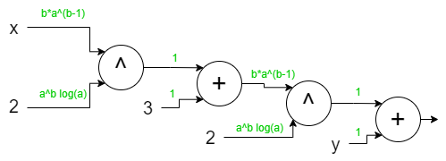
We are almost done. The only thing we need to do now is multiply the edges between the output and the variable you want to find its derivative.
If we want to find the derivative of y, then it’s simply 1 because there is a single edge between it and the output, and it’s 1.
For the derivative of x, it will be starting from right to left:
\[1\cdot(b_0a_0^{b_0-1})\cdot 1\cdot (b_1a_1^{b_1-1})\]Just follow the edges to x starting from the output of the graph. I know this looks hard, but don’t forget that computers will do this, not you :) Now we need to substitute the a0, b0, a1 and b0. For this we add one more thing to do edges, results they carry:
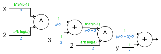
Each upper edge is an a, and each lower edge is a b:
\[a_0 = x \ \ \ \ \ \ b_0 = 2 \ \ \ \ \ \ a_1 = x^2+3 \ \ \ \ \ \ b_1 = 2\]When we substitute we get:
\[4x(x^2+3)\]This is true if you check it from the WolframAlpha.
This method we learned is called backpropagation. This is the core of all neural network libraries. Now we’ll understand why this works.
There is a concept called Chain rule in calculus. It looks like this:
\[\frac{\partial z}{\partial x} = \frac{\partial z}{\partial y} \cdot \frac{\partial y}{\partial x}\]This rule says that we can compose basic operation derivatives to get the full derivative, which is what we have done
so far. We multiplied basic derivatives for f = (x^2 + 3)^2 + y. You can see this by giving names to each node output
that goes to x:
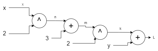
This can be now translated to chain rule as:
\[\frac{\partial L}{\partial x} = \frac{\partial L}{\partial k} \cdot \frac{\partial k}{\partial m} \cdot \frac{\partial m}{\partial n} \cdot \frac{\partial n}{\partial x}\]If you understand this, then the rest is a piece of cake.
Now it’s time for implementation. First, let’s create a new class for the variables and construct the graph as we operate on them:
class Var:
    def __init__(self, value, requires_grad=False, prev_var1=None, prev_var2=None, prev_op=None):
        self.value = value
        self.requires_grad = requires_grad
        if requires_grad:
            self.grad = 0

        self.prev_var1 = prev_var1
        self.prev_var2 = prev_var2
        self.prev_op = prev_op

    def __add__(self, other):
        return Var(self.value + other.value, prev_var1=self, prev_var2=other, prev_op="add")

    def __mul__(self, other):
        return Var(self.value * other.value, prev_var1=self, prev_var2=other, prev_op="mul")

    def __pow__(self, other):
        return Var(self.value**other.value, prev_var1=self, prev_var2=other, prev_op="pow")

    def backward(self, current_grad=1):
        if self.prev_op == "add":
            self.prev_var1.backward(current_grad)
            self.prev_var2.backward(current_grad)
        elif self.prev_op == "mul":
            self.prev_var1.backward(current_grad * self.prev_var2.value)
            self.prev_var2.backward(current_grad * self.prev_var1.value)
        elif self.prev_op == "pow":
            self.prev_var1.backward(
                current_grad * self.prev_var2.value * self.prev_var1.value ** (self.prev_var2.value - 1)
            )
            self.prev_var2.backward(
                current_grad * self.prev_var1.value**self.prev_var2.value * math.log(self.prev_var1.value)
            )
        elif self.prev_op is None:
            pass
        else:
            assert False, "No such operation"

        if self.requires_grad:
            self.grad += current_grad
Let’s understand this code. Every variable can be composed of two previous variables and an operation, like for z = x + y, prev_var1 is x, prev_var2 is y and the operation is add operation.
We have the __add__, __mul__ and __pow__ functions. These are Python magic functions. If we have something like:
x = Var(3)
y = Var(4)

z = x + y
Then the __add__ function of the Variable x will be called. z will have x and y as it’s previous variables and
its value will be x.value + y.value.
The fun part is the backward function. This function will calculate the derivative for all variables that are
a part of the computation graph and has the attribute requires_grad.
Let’s go through this function step-by-step for the (x**2 + 3)**2 + y.
x = Var(53)
y = Var(-17)

z = (x**2 + 3)**2 + y
z.backward()

print(x.grad)
print(y.grad)z’s last operation is add, so when the z.backward() called, it will recursively call the backward for prev_var1
and prev_var2. prev_var1 is (x**2 + 3)**2 and prev_var2 is y. We will accumulate the derivative at the
current_grad variable. It will basically be accumulated by derivatives we found for add, multiply, and power operations.
If you are having a hard time understanding the backward function, you should take a look at algorithms
like DFS and maybe try learning a bit more about processing the graphs. I will not go into the depth of this as
I already visually demonstrated what this function does. So you know what’s going on.
Now, if you try to run the last code block, you will notice that it will throw an error. The reason is after we call
x**2, __add__ function will try to access the value attribute for the number 2, which has no such attribute
since it is just a basic type of integer.
To fix this we need to convert any value to Var if it already isn’t. And before giving the full code, we will also
take into consideration the operations like 2 + x. This would also throw an error since this won’t be calling the __add__
function of the Var class. It should strictly be after the x, like x + 2. To fix it we need to add some other
magic function.
class Var:
    def __init__(self, value, requires_grad=False, prev_var1=None, prev_var2=None, prev_op=None):
        self.value = value
        self.requires_grad = requires_grad
        if requires_grad:
            self.grad = 0

        self.prev_var1 = prev_var1
        self.prev_var2 = prev_var2
        self.prev_op = prev_op

    def __add__(self, other):
        if not isinstance(other, Var):
            other = Var(other)

        return Var(self.value + other.value, prev_var1=self, prev_var2=other, prev_op="add")

    def __mul__(self, other):
        if not isinstance(other, Var):
            other = Var(other)

        return Var(self.value * other.value, prev_var1=self, prev_var2=other, prev_op="mul")

    def __pow__(self, other):
        if not isinstance(other, Var):
            other = Var(other)

        return Var(self.value**other.value, prev_var1=self, prev_var2=other, prev_op="pow")

    def __rpow__(self, other):
        if not isinstance(other, Var):
            other = Var(other)

        return Var(other.value**self.value, prev_var1=other, prev_var2=self, prev_op="pow")

    def __radd__(self, other):
        # for operations like 2+x
        return self + other

    def __sub__(self, other):
        # for operations like x-2
        return self + (-other)

    def __rsub__(self, other):
        # for operations like 2-x
        return other + (-self)

    def __neg__(self):
        # for operations like -x
        return self * -1

    def __rmul__(self, other):
        # for operations like 2*x
        return self * other

    def __truediv__(self, other):
        # for operations like x/2
        return self * other**-1

    def __rtruediv__(self, other):
        # for operations like 2/x
        return other * self**-1

    def backward(self, current_grad=1):
        if self.prev_op == "add":
            self.prev_var1.backward(current_grad)
            self.prev_var2.backward(current_grad)
        elif self.prev_op == "mul":
            self.prev_var1.backward(current_grad * self.prev_var2.value)
            self.prev_var2.backward(current_grad * self.prev_var1.value)
        elif self.prev_op == "pow":
            self.prev_var1.backward(
                current_grad * self.prev_var2.value * self.prev_var1.value ** (self.prev_var2.value - 1)
            )
            self.prev_var2.backward(
                current_grad * self.prev_var1.value**self.prev_var2.value * math.log(self.prev_var1.value)
                if self.prev_var1.value > 0
                else 0
            )
        elif self.prev_op == "sigmoid":
            self.prev_var1.backward(
                current_grad * self.prev_var1.sigmoid().value * (1 - self.prev_var1.sigmoid().value)
            )
        elif self.prev_op is None:
            pass
        else:
            assert False, "No such operation"

        if self.requires_grad:
            self.grad += current_grad
Congratulations! You just implemented the backpropagation algorithm!
But before continuing, you might have worried about the derivatives if we had an equation like:
\[(x^2 + 3) ^ 2 + x\]Now the last y became x. And if we look at the computation graph it will have two different x fed into the graph:
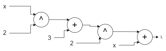
We will get two different derivatives for x since there are two paths to x from the output. For this,
we will simply add those derivatives. The implementation has already been doing this by self.grad += current_grad.
This also comes from the chain rule, which can also be written as:
\[\frac{\partial z}{\partial x} = \frac{\partial z}{\partial y} \cdot \frac{\partial y}{\partial x} + \frac{\partial z}{\partial w} \cdot \frac{\partial w}{\partial x}\]5. Update the parameters by subtracting their scaled derivatives
With the backpropagation algorithm done, we can get the derivatives for each of our parameters by calling the
loss.backward(). It will calculate the derivative for each of the parameters. Now we will use these
derivatives to update the actual value of the parameters.
Before that need to talk about one more simple thing, the scaled term in the title. We can’t simply subtract the gradient from the parameter’s value. We need to scale the gradient. This is because the gradients can be too big which can hurt the training. We want to go in that direction, not by that exact amount.
We achieve this scaling by something called learning rate that we multiply our derivatives before subtracting. It is usually set to values like 0.001. But there is no formula for it, you need to adjust them until you find a good value.
Let’s finish our AND example by re-defining our NN class:
class NN:
    def __init__(self):
        self.parameters = []
        for _ in range(3):
            var = Var(random.random(), requires_grad=True)
            self.parameters.append(var)

    def sigmoid(self, x):
        return 1 / (1 + math.e ** (-x))

    def forward(self, p, q):
        out1 = p * self.parameters[0]
        out2 = q * self.parameters[1]
        output = self.sigmoid(out1 + out2 + self.parameters[2])

        return output

    def calculate_loss(self, data):
        loss = 0
        for d in data:
            bit1, bit2 = d[0], d[1]
            prediction = self.forward(bit1, bit2)

            real_value = d[2]
            loss += (prediction - real_value) ** 2

        return loss

data = [
    [0, 0, 0],
    [0, 1, 0],
    [1, 0, 0],
    [1, 1, 1],
]

model = NN()
lr = 0.1

for _ in range(1000):
    loss = model.calculate_loss(data)
    print(f"loss: {loss.value}")
    loss.backward()

    for i in range(len(model.parameters)):
        model.parameters[i].value -= lr * model.parameters[i].grad
        model.parameters[i].grad = 0

for d in data:
    bit1, bit2 = d[0], d[1]
    prediction = model.forward(bit1, bit2).value

    print(f"{bit1} & {bit2} = {prediction}")
And here it is! We have successfully trained our network for the AND gate. If you run it you will see it correctly predicts the bits.
Now let’s try the XOR gate as our data:
data = [
    [0, 0, 0],
    [0, 1, 1],
    [1, 0, 1],
    [1, 1, 0],
]
We keep everything rest the same, and run again, but we fail to learn this time. The network predicts 0.5 for every input. The reason is our network is simply not capable of representing the XOR gate.
We will fix this by adding additional layers to our network model. Until now, our neural network looked something like this:
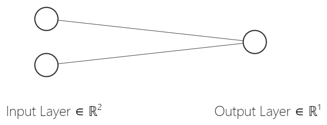
Each edge shows our weights (parameters 1 and 2), and we add bias (parameter 3) at the output layer.
To increase the capabilities of our network, we will simply add a hidden layer. So it will look like:
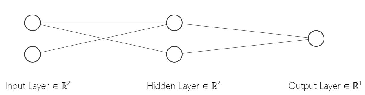
We could even add more layers and each layer can have any number of nodes:
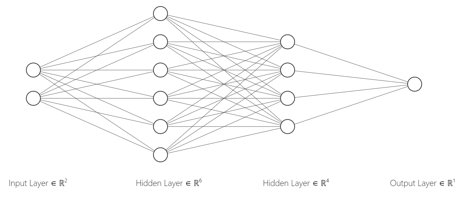
We need a different parameter for each edge now, and for non-input layers, we will need biases for each node. These nodes at the non-input layers are called neurons. We can have as many neurons and layers in neural networks. In the last figure, there are 6 neurons in the first hidden layer and 4 neurons in the second hidden layer. An important part here is that we need to use the activation functions after every layer.
The reason we need this is that if we don’t do that, extra layers will lose all the benefits they add. Because without non-linear functions it’s all multiplying and adding. Even if you have 1000 layers, without non-linearity they all can be simplified to a single layer. If you take any number and multiply it with thousands of numbers and add thousands of numbers, the same result can be simplified to multiplying it with a single number and adding a single number:
\[(((xa + b)c + d)e + f) = xg + h\]So we need activation functions after calculating the value for every neuron.
Let’s get back to implementation. We can generalize our neural network implementation to be flexible for any type of architecture easily, but this is not related to this tutorial. It simply requires many loops. But I will give you a repository at the end if you want to see how you can implement it.
Now our network instead will have one additional hidden layer with two neurons. It will have a total of 9 parameters:
class NN:
    def __init__(self):
        self.weights1 = [Var(random.random(), requires_grad=True), Var(random.random(), requires_grad=True)]
        self.bias1 = Var(random.random(), requires_grad=True)

        self.weights2 = [Var(random.random(), requires_grad=True), Var(random.random(), requires_grad=True)]
        self.bias2 = Var(random.random(), requires_grad=True)

        self.weights3 = [Var(random.random(), requires_grad=True), Var(random.random(), requires_grad=True)]
        self.bias3 = Var(random.random(), requires_grad=True)

        self.parameters = [
            *self.weights1,
            self.bias1,
            *self.weights2,
            self.bias2,
            *self.weights3,
            self.bias3,
        ]

    def sigmoid(self, x):
        return 1 / (1 + math.e ** (-x))

    def forward(self, p, q):
        out1 = p * self.weights1[0] + q * self.weights1[1] + self.bias1
        out1 = self.sigmoid(out1)

        out2 = p * self.weights2[0] + q * self.weights2[1] + self.bias2
        out2 = self.sigmoid(out2)

        out3 = out1 * self.weights3[0] + out2 * self.weights3[1] + self.bias3
        output = self.sigmoid(out3)

        return output

    def calculate_loss(self, data):
        loss = 0
        for d in data:
            bit1, bit2 = d[0], d[1]
            prediction = self.forward(bit1, bit2)

            real_value = d[2]
            loss += (prediction - real_value) ** 2

        return loss
Now if you increase the learning rate to 1 (it is actually a pretty big for a learning rate but works well in this example), and increase the number of iterations to 2000, you’ll see it learns the XOR gate in a couple of seconds!
Here is the full code in a single file: https://gist.github.com/anilzeybek/3e96b4fc48e59612dc3f56586b233718.
Here is a repository that includes both backprop and finite difference implementations and NN implementation that can represent any number of layers and neurons, as well as a PyTorch implementation: https://github.com/anilzeybek/nn-from-scratch.
If you’ve managed to read this far, congratulations. Now you know how the neural networks work. As simple as they are, they are extremely powerful. Good luck to you in your future studies.